Reconstructing a plot from the National Weather Service
A no-so-great graphic
It’s been snowing a lot lately in Iowa, so someone sent me this tweet about just how much snow we’ve been getting. Instead of getting shocked at the snow, I was shocked at the data visualization.
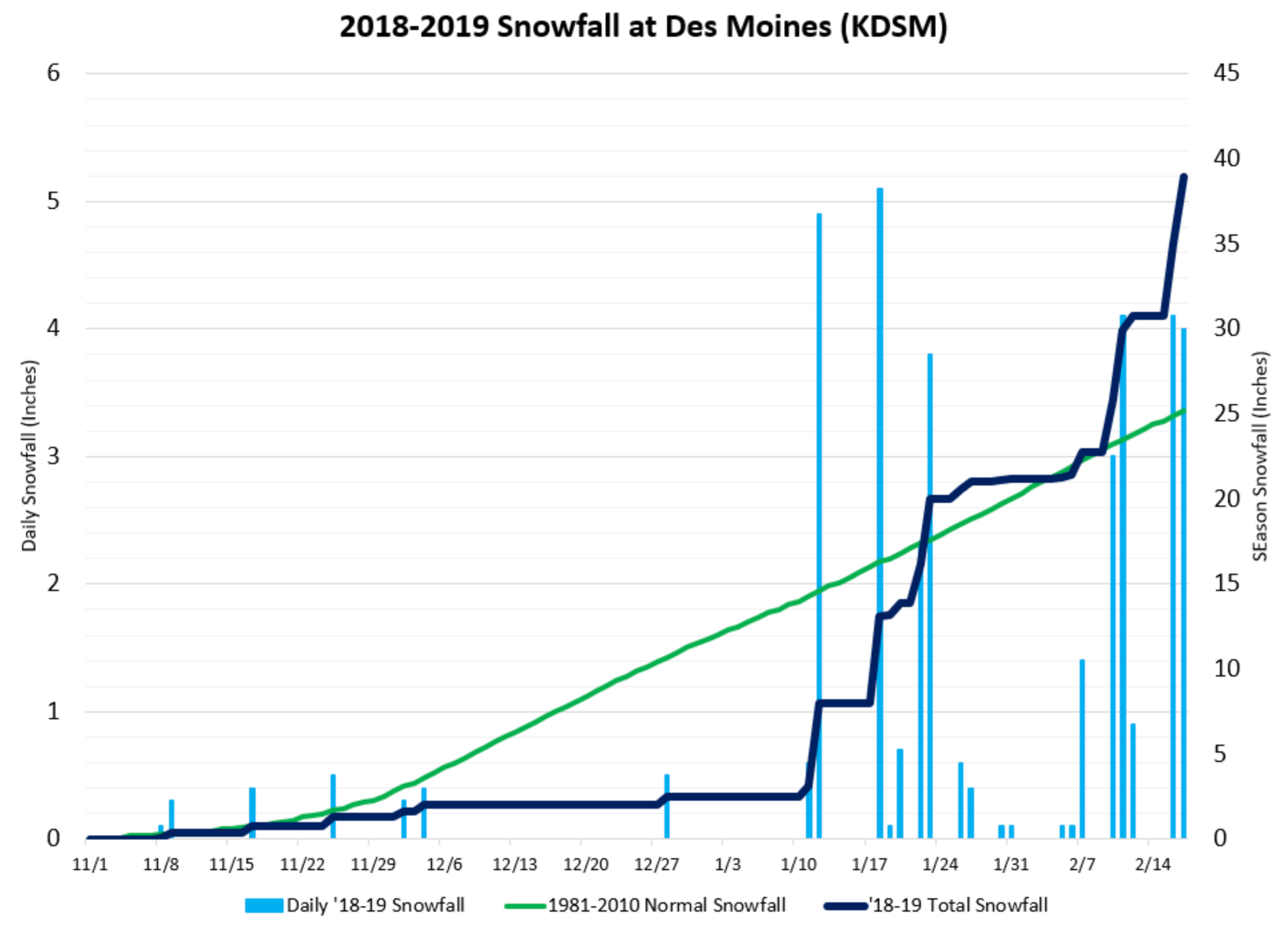
Why is this graphic not so great? Mostly, the double y-axis is very misleading. On 1/18, it looks like we got more snow in one day than we did all winter! So, with another snowy day again today, I decided to re-make it without the dual y-axes.
Making a better graphic
The National Weather Service takes in data from NOAA. So, I went searching for an R package for getting NOAA data into R. Luckily, rOpenSci has one! It’s called rnoaa. What follows is how I got the data and re-created the graphic.
First, attach the necessary packages.
# install.packages("rnoaa")
library(rnoaa)
library(tidyverse)
Then, get an API token for the NOAA APIs. (Mine took about 20 minutes to come through.) Once you have that, set it up in your R session with options():
options(noaakey = "YOUR_KEY")Next, find the Des Moines weather station(s) that will have the recorded data we want (historical daily snowfall).
# all stations with historical data
stat <- ghcnd_stations()head(stat)## # A tibble: 6 x 11
## id latitude longitude elevation state name gsn_flag wmo_id element
## <chr> <dbl> <dbl> <dbl> <chr> <chr> <chr> <dbl> <chr>
## 1 ACW0… 17.1 -61.8 10.1 <NA> ST J… <NA> NA TMAX
## 2 ACW0… 17.1 -61.8 10.1 <NA> ST J… <NA> NA TMIN
## 3 ACW0… 17.1 -61.8 10.1 <NA> ST J… <NA> NA PRCP
## 4 ACW0… 17.1 -61.8 10.1 <NA> ST J… <NA> NA SNOW
## 5 ACW0… 17.1 -61.8 10.1 <NA> ST J… <NA> NA SNWD
## 6 ACW0… 17.1 -61.8 10.1 <NA> ST J… <NA> NA PGTM
## # … with 2 more variables: first_year <dbl>, last_year <dbl>stat %>% filter(str_detect(name, "MOINES")) %>% # look for "des moines"
arrange(first_year, desc(last_year)) %>% # make sure the years we want are covered (1981-2010, 2018-2019)
filter(element == "SNOW") # we need snowfall data## # A tibble: 25 x 11
## id latitude longitude elevation state name gsn_flag wmo_id element
## <chr> <dbl> <dbl> <dbl> <chr> <chr> <chr> <dbl> <chr>
## 1 USC0… 36.8 -104. 2018. NM DES … <NA> NA SNOW
## 2 USC0… 36.8 -104. 1830 NM DES … <NA> NA SNOW
## 3 USW0… 41.5 -93.7 292. IA DES … GSN 72546 SNOW
## 4 USC0… 41.6 -93.6 248. IA DES … <NA> NA SNOW
## 5 USC0… 41.6 -93.6 252. IA DES … <NA> NA SNOW
## 6 USC0… 41.7 -93.7 292. IA DES … <NA> NA SNOW
## 7 US1I… 41.6 -93.7 261. IA DES … <NA> NA SNOW
## 8 US1N… 36.6 -104. 1990 NM DES … <NA> NA SNOW
## 9 US1I… 41.6 -93.7 258. IA DES … <NA> NA SNOW
## 10 US1I… 41.6 -93.8 278 IA WEST… <NA> NA SNOW
## # … with 15 more rows, and 2 more variables: first_year <dbl>, last_year <dbl>dsm_info <- stat %>% filter(str_detect(name, "MOINES")) %>%
arrange(first_year, desc(last_year)) %>%
filter(element == "SNOW") %>% slice(3) # 3rd row is actually DSM, IA, and has 70+ years of data
dsm_id <- dsm_info %>% pull(id) # get the ID for this weather stationAfter a few failed attempts, and reading the rnoaa documentation, I decided that the best data source would be the Global Historical Climatology Network daily weather data. These data are documented here. The ghcnd() function gets all weather data for a particular station.
hist_dsm_data <- ghcnd(dsm_id, refresh = TRUE)
head(hist_dsm_data)
## # A tibble: 6 x 128
## id year month element VALUE1 MFLAG1 QFLAG1 SFLAG1 VALUE2 MFLAG2 QFLAG2
## <chr> <dbl> <dbl> <chr> <dbl> <lgl> <lgl> <chr> <dbl> <lgl> <lgl>
## 1 USW0… 1945 7 TMAX 217 NA NA X 244 NA NA
## 2 USW0… 1945 7 TMIN 128 NA NA X 100 NA NA
## 3 USW0… 1945 7 PRCP 0 NA NA X 0 NA NA
## 4 USW0… 1945 7 SNOW 0 NA NA X 0 NA NA
## 5 USW0… 1945 7 WT01 NA NA NA <NA> NA NA NA
## 6 USW0… 1945 7 WT03 NA NA NA <NA> NA NA NA
## # … with 117 more variables: SFLAG2 <chr>, VALUE3 <dbl>, MFLAG3 <lgl>,
## # QFLAG3 <lgl>, SFLAG3 <chr>, VALUE4 <dbl>, MFLAG4 <lgl>, QFLAG4 <lgl>,
## # SFLAG4 <chr>, VALUE5 <dbl>, MFLAG5 <lgl>, QFLAG5 <lgl>, SFLAG5 <chr>,
## # VALUE6 <dbl>, MFLAG6 <lgl>, QFLAG6 <lgl>, SFLAG6 <chr>, VALUE7 <dbl>,
## # MFLAG7 <lgl>, QFLAG7 <lgl>, SFLAG7 <chr>, VALUE8 <dbl>, MFLAG8 <lgl>,
## # QFLAG8 <lgl>, SFLAG8 <chr>, VALUE9 <dbl>, MFLAG9 <lgl>, QFLAG9 <lgl>,
## # SFLAG9 <chr>, VALUE10 <dbl>, MFLAG10 <lgl>, QFLAG10 <lgl>, SFLAG10 <chr>,
## # VALUE11 <dbl>, MFLAG11 <lgl>, QFLAG11 <lgl>, SFLAG11 <chr>, VALUE12 <dbl>,
## # MFLAG12 <lgl>, QFLAG12 <lgl>, SFLAG12 <chr>, VALUE13 <dbl>, MFLAG13 <lgl>,
## # QFLAG13 <lgl>, SFLAG13 <chr>, VALUE14 <dbl>, MFLAG14 <lgl>, QFLAG14 <lgl>,
## # SFLAG14 <chr>, VALUE15 <dbl>, MFLAG15 <lgl>, QFLAG15 <lgl>, SFLAG15 <chr>,
## # VALUE16 <dbl>, MFLAG16 <lgl>, QFLAG16 <lgl>, SFLAG16 <chr>, VALUE17 <dbl>,
## # MFLAG17 <lgl>, QFLAG17 <lgl>, SFLAG17 <chr>, VALUE18 <dbl>, MFLAG18 <lgl>,
## # QFLAG18 <lgl>, SFLAG18 <chr>, VALUE19 <dbl>, MFLAG19 <chr>, QFLAG19 <lgl>,
## # SFLAG19 <chr>, VALUE20 <dbl>, MFLAG20 <lgl>, QFLAG20 <lgl>, SFLAG20 <chr>,
## # VALUE21 <dbl>, MFLAG21 <lgl>, QFLAG21 <lgl>, SFLAG21 <chr>, VALUE22 <dbl>,
## # MFLAG22 <lgl>, QFLAG22 <lgl>, SFLAG22 <chr>, VALUE23 <dbl>, MFLAG23 <lgl>,
## # QFLAG23 <lgl>, SFLAG23 <chr>, VALUE24 <dbl>, MFLAG24 <lgl>, QFLAG24 <lgl>,
## # SFLAG24 <chr>, VALUE25 <dbl>, MFLAG25 <lgl>, QFLAG25 <lgl>, SFLAG25 <chr>,
## # VALUE26 <dbl>, MFLAG26 <lgl>, QFLAG26 <lgl>, SFLAG26 <chr>, VALUE27 <dbl>,
## # MFLAG27 <lgl>, QFLAG27 <lgl>, …And now we corral the data for the visualization! We need (in inches):
- Daily snowfall amounts for the current winter
- Historical average daily snowfall amounts for the 1981-2010 winters
- Cumulative amounts of 1 and 2.
The data are very wide, with 3 columns for each day of the month.
# make wide data long
wide_to_long <- hist_dsm_data %>% filter(element=="SNOW") %>%  # just want snowfall totals
  select(year, month,starts_with("VALUE")) %>% # per documentation, VALUE# indicates the day of the month
  gather(day, fall_mm, VALUE1:VALUE31) %>% # go from wide to long
  mutate(day = parse_number(day)) %>% # convert day to a number
  filter(!is.na(day)) # get rid of days that are missing/don't exist
head(wide_to_long)
## # A tibble: 6 x 4
## year month day fall_mm
## <dbl> <dbl> <dbl> <dbl>
## 1 1945 7 1 0
## 2 1945 8 1 0
## 3 1945 9 1 0
## 4 1945 10 1 0
## 5 1945 11 1 0
## 6 1945 12 1 0# get winter data
winter_data <- wide_to_long %>%
mutate(date = lubridate::make_date(year = year, month = month, day = day)) %>% # create an actual date column
arrange(date) %>%
filter(!is.na(fall_mm)) %>% # remove missings e.g. for February 30th
filter(month %in% c(11, 12, 1, 2))# only want winter months
head(winter_data)## # A tibble: 6 x 5
## year month day fall_mm date
## <dbl> <dbl> <dbl> <dbl> <date>
## 1 1945 11 1 0 1945-11-01
## 2 1945 11 2 0 1945-11-02
## 3 1945 11 3 0 1945-11-03
## 4 1945 11 4 0 1945-11-04
## 5 1945 11 5 0 1945-11-05
## 6 1945 11 6 0 1945-11-06# get cumulative totals
snow_data_hist <- winter_data %>%
mutate(year2 = ifelse(month %in% c(1,2), year-1, year)) %>% # create another year variable to group by
arrange(date) %>%
group_by(year2) %>% # so we can get cumulative snowfall in a winter season, not in a calendar year.
mutate(fall_mm_cum = cumsum(fall_mm)) # compute cumulative snowfall
head(snow_data_hist)## # A tibble: 6 x 7
## # Groups: year2 [1]
## year month day fall_mm date year2 fall_mm_cum
## <dbl> <dbl> <dbl> <dbl> <date> <dbl> <dbl>
## 1 1945 11 1 0 1945-11-01 1945 0
## 2 1945 11 2 0 1945-11-02 1945 0
## 3 1945 11 3 0 1945-11-03 1945 0
## 4 1945 11 4 0 1945-11-04 1945 0
## 5 1945 11 5 0 1945-11-05 1945 0
## 6 1945 11 6 0 1945-11-06 1945 0# get date ranges to match original plot
avg_81_10 <- filter(snow_data_hist, year2 %in% 1981:2010)
head(avg_81_10)## # A tibble: 6 x 7
## # Groups: year2 [1]
## year month day fall_mm date year2 fall_mm_cum
## <dbl> <dbl> <dbl> <dbl> <date> <dbl> <dbl>
## 1 1981 11 1 0 1981-11-01 1981 0
## 2 1981 11 2 0 1981-11-02 1981 0
## 3 1981 11 3 0 1981-11-03 1981 0
## 4 1981 11 4 0 1981-11-04 1981 0
## 5 1981 11 5 0 1981-11-05 1981 0
## 6 1981 11 6 0 1981-11-06 1981 0# compute daily averages over the 30 year period
snow_data_avg <- avg_81_10 %>% ungroup() %>% group_by(day, month) %>%
mutate(avg_c_sum = mean(fall_mm_cum), avg_day_mm = mean(fall_mm))
# make sure date ranges match data available for 2019
snow_data_avg2 <- snow_data_avg %>% select(month, day, avg_c_sum, avg_day_mm) %>%
unique() %>% filter(month != 2 | !(month == 2 & day >16))
thisyear <- filter(snow_data_hist, year2 == 2018)
head(thisyear) ## # A tibble: 6 x 7
## # Groups: year2 [1]
## year month day fall_mm date year2 fall_mm_cum
## <dbl> <dbl> <dbl> <dbl> <date> <dbl> <dbl>
## 1 2018 11 1 0 2018-11-01 2018 0
## 2 2018 11 2 0 2018-11-02 2018 0
## 3 2018 11 3 0 2018-11-03 2018 0
## 4 2018 11 4 0 2018-11-04 2018 0
## 5 2018 11 5 0 2018-11-05 2018 0
## 6 2018 11 6 0 2018-11-06 2018 0thisyear %>% left_join(snow_data_avg2) %>% head() # combine historical data with this year's data## # A tibble: 6 x 9
## # Groups: year2 [1]
## year month day fall_mm date year2 fall_mm_cum avg_c_sum avg_day_mm
## <dbl> <dbl> <dbl> <dbl> <date> <dbl> <dbl> <dbl> <dbl>
## 1 2018 11 1 0 2018-11-01 2018 0 1.53 1.53
## 2 2018 11 2 0 2018-11-02 2018 0 3 1.47
## 3 2018 11 3 0 2018-11-03 2018 0 3.33 0.333
## 4 2018 11 4 0 2018-11-04 2018 0 3.5 0.167
## 5 2018 11 5 0 2018-11-05 2018 0 5.37 1.87
## 6 2018 11 6 0 2018-11-06 2018 0 9.37 4Finally, re-do the plot with a single y-axis. I also added daily average snowfall in red to compare the daily totals with this year’s daily snowfall.
p <- thisyear %>% left_join(snow_data_avg2) %>%
  ggplot(aes(x = date)) +
  geom_line(aes(y = avg_c_sum*0.0393701, color = "1981-2010 Normal Snowfall"), size = 1.5)  + # multiply by 0.0393701 to convert mm to in
  geom_line(aes(y = fall_mm_cum*0.0393701, color = "2018-19 Total Snowfall"), size = 1.5) +
  geom_segment(aes(x = date, xend = date, y = 0, yend = fall_mm*0.0393701, color ="2018-19 Daily Snowfall"), size = 1.5) +
  geom_segment(aes(x = date, xend = date, y = 0, yend = avg_day_mm*0.0393701, color ="1981-2010 Average Daily Snowfall"), size = 1.5, alpha = .7) +
  labs(x = "Date", y = "Snowfall (in)", title = "2018-19 Snowfall in Des Moines") +
  scale_x_date(date_breaks = "1 weeks", date_labels = "%m/%d") +
  scale_y_continuous(breaks = 0:7*5, position = "right") +
  theme_bw() +
  scale_color_manual(name = "", values = c("2018-19 Daily Snowfall" = "#00B0F0",
                                           "1981-2010 Normal Snowfall" = "#00B050",
                                           "2018-19 Total Snowfall" = "navy",
                                           "1981-2010 Average Daily Snowfall" = "#71e8a7"),
                     guide = guide_legend(nrow = 2)) +
  theme(legend.position = "bottom", plot.title = element_text(face = "bold", hjust = .5))
p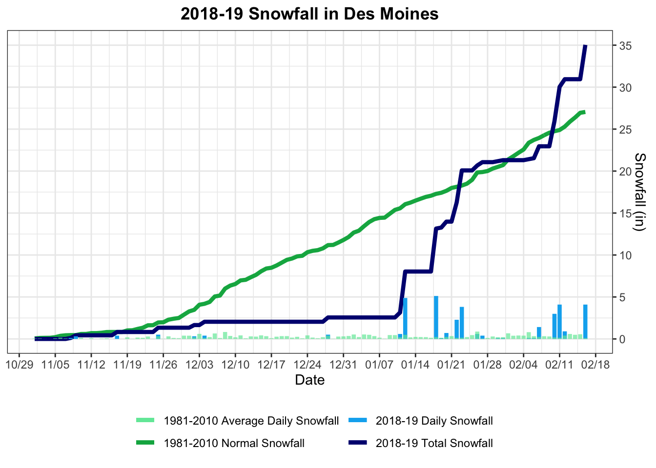
So, what do you think?
or

Addendum
Today, I learned different having a different geom_*s in each facet panel is a thing!
I’d wonder about putting the daily snow fall in a different facet and using scales = “free” (different geoms in different facets is a cool trick that I don’t think enough people know about)
— Hadley Wickham (@hadleywickham) February 21, 2019
My solution. Thanks to this StackOverflow question.
snowdata <- thisyear %>% left_join(snow_data_avg2)
snowdata2 <- snowdata %>%
  gather(type, mm_snow, c(fall_mm, fall_mm_cum:avg_day_mm))

snowdata2 <- snowdata2 %>%
  mutate(type2 = recode(type, fall_mm = "Daily", fall_mm_cum = "Cumulative Snowfall",
                        avg_c_sum = "Cumulative Snowfall", avg_day_mm = "Daily"),
         in_snow = mm_snow * 0.0393701)
head(snowdata2)
## # A tibble: 6 x 9
## # Groups: year2 [1]
## year month day date year2 type mm_snow type2 in_snow
## <dbl> <dbl> <dbl> <date> <dbl> <chr> <dbl> <chr> <dbl>
## 1 2018 11 1 2018-11-01 2018 fall_mm 0 Daily 0
## 2 2018 11 2 2018-11-02 2018 fall_mm 0 Daily 0
## 3 2018 11 3 2018-11-03 2018 fall_mm 0 Daily 0
## 4 2018 11 4 2018-11-04 2018 fall_mm 0 Daily 0
## 5 2018 11 5 2018-11-05 2018 fall_mm 0 Daily 0
## 6 2018 11 6 2018-11-06 2018 fall_mm 0 Daily 0ggplot() +
geom_line(data = snowdata2 %>% filter(type2 == "Cumulative Snowfall"), aes(x = date, y = in_snow, color = type), size = 1.5) +
geom_bar(data = snowdata2 %>% filter(type2 == "Daily"), aes(x = date, weight = in_snow, fill = type), size = 1.5, position = "dodge") +
scale_color_brewer(palette = "Paired") +
scale_fill_brewer(name = "", palette = "Paired", labels = c("1981-2010 Average Snowfall", "2018-2019 Snowfall")) +
scale_x_date(name = "Date (winter 2018-19)", breaks = "1 week", date_labels = "%m/%d") +
labs(y= "Snowfall in Inches", title = "2018-19 Snowfall in Des Moines") +
guides(color = "none") +
theme_bw() +
theme(legend.position = "bottom", plot.title = element_text(face = "bold", hjust = .5), aspect.ratio = .4,
axis.text.x = element_text(angle = 45, hjust = 1)) +
facet_wrap(~type2, nrow = 1, scales = "free_y" )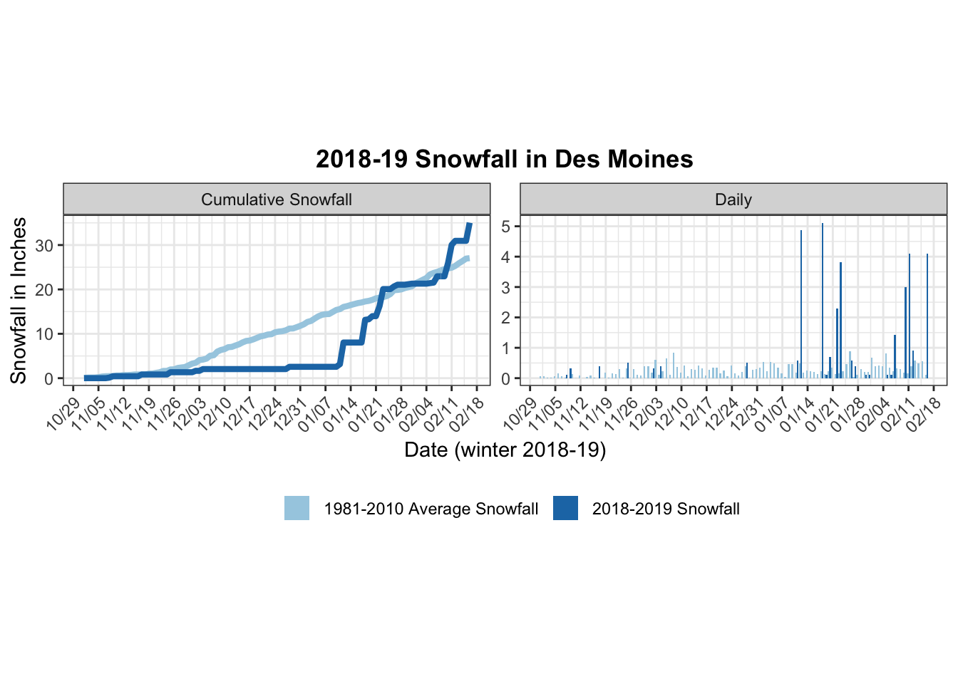
ggplot() +
  geom_line(data = snowdata2 %>% filter(type2 == "Cumulative Snowfall"), aes(x = date, y = in_snow, color = type), size = 1.5) +
  geom_bar(data = snowdata2 %>% filter(type2 == "Daily"), aes(x = date, weight = in_snow, fill = type), size = 1.5, position = "dodge")  +
  scale_color_brewer(palette = "Paired") +
  scale_fill_brewer(name = "", palette = "Paired", labels = c("1981-2010 Average Snowfall", "2018-2019 Snowfall")) +
  scale_x_date(name = "Date (winter 2018-19)", breaks = "1 week", date_labels = "%m/%d") +
  labs(y= "Snowfall in Inches", title = "2018-19 Snowfall in Des Moines") +
  guides(color = "none") +
  theme_bw() +
  theme(legend.position = "bottom", plot.title = element_text(face = "bold", hjust = .5),
        axis.text.x = element_text(angle = 45, hjust = 1)) +
  facet_grid(type2~., space = "free", scales = "free_y")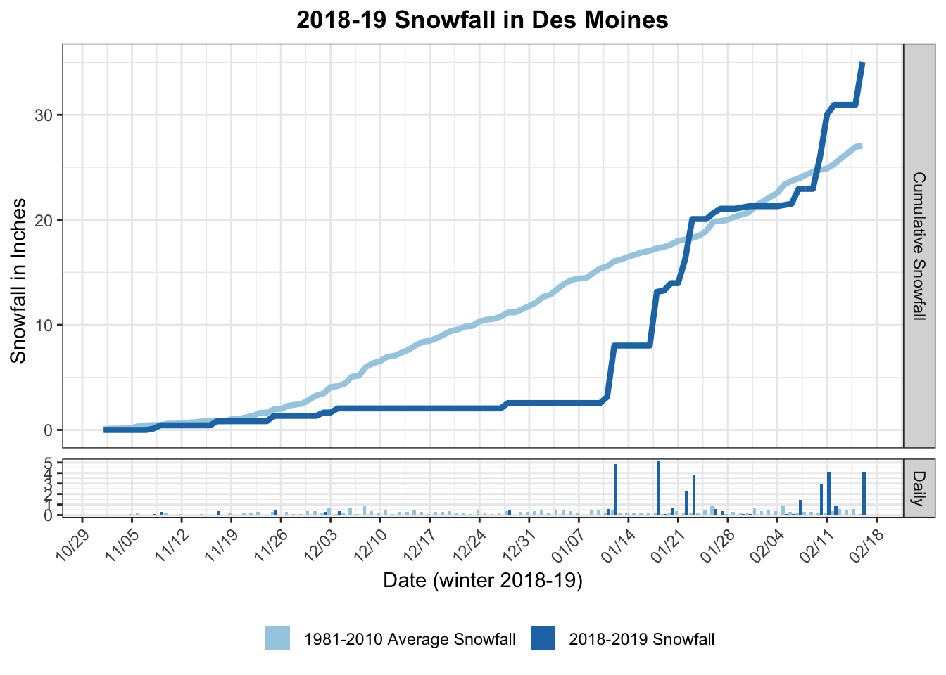
Sam Tyner-Monroe, Ph.D.
Managing Director, Responsible AI
I am an applied statistician and data scientist, with a wide range of skills and experiences. I’m passionate about using data to make a difference.