Forensic Glass Analysis - Part I
What is the forensic problem at hand?
It is easy to imagine a crime scene with glass fragments: a burglar may have broken a glass door, a glass bottle could have been used in an assault, or a domestic disturbance may involve throwing something through a window. There are many ways that glass can break and that glass fragments can be transferred. The study of glass fragments is important to forensic science because the glass broken at the scene can transfer to the perpetrator’s shoes, clothing, or even their hair [1].
Crime scene investigators collect fragments of glass at the scene as a part of the evidence collection process and the fragments are sent to the forensics lab for processing. Similarly, evidence such as clothing and shoes are collected from a suspect, and if glass is found, the fragments are compared to the fragments found at the scene. We refer to the relevant measurements/observations of the crime scene glass as \(G_C\) for Glass from the Crime scene. In cases like these, some glass fragments are found on the suspect’s clothing or perhaps in the suspect’s vehicle. The amount of glass found on the suspect is usally much smaller than the amount available from the scene for testing and analysis. Thus, after the relevant measurements/observations from the suspect, \(G_S\), are made, the glass that was found on the suspect is often destroyed. The fundamental forensic task at hand is to determine if the source of the glass found on the suspect is the window from the crime scene or another, unknown source. This is generally broadened and formalized as a pair of competing hypotheses written in terms of the measurements on the two glass sources:
\[ \begin{align*} H_0 & : \quad G_C \text{ and } G_S \text{ come from the same source} \\ H_1 & : \quad G_C \text{ and } G_S \text{ come from different sources} \end{align*} \]
The forensic expert analyzes samples from the two sources, \(C\) and \(S\) for crime scene and suspect, respectively, obtaining the measurements \(G_C\) and \(G_S\). Then, the expert makes a comparison following a pre-defined methodology to determine whether or not \(G_C\) and \(G_S\) come from the same source.
This type of problem fits into the “source level” type of hypothesis. The goal of the source level hypothesis is to determine if the “suspect” is the source of the “evidence” (e.g. the glass found on the suspect is from the same source as the glass at the scene). Typically, this is the “lowest level” of hypothesis in a crime investigation. The other levels are “activity level” and “offence level”. Activity level hypotheses concern whether the “suspect” created or caused the “evidence” (e.g. the suspect broke the window at the scene). Offense level hypotheses go one step further, determining whether or not the “suspect” committed the “crime” (e.g. the suspect committed the robbery). For more on the different types of hypotheses, see Cook et al. [2]
Glass element analysis
Float glass is made from a molten mixture of silica sand, soda ash (sodium carbonate [\(Na_2 CO_3\)]), limestone, dolomite [\(CaMg(CO_3)_2\)], salt cake (sodium sulfate [\(Na_2SO_4\)]), waste glass from previous runs, and other materials. The amounts of these compunds in glass are known to vary by manufacturer and how much material is available at the time. The materials are melted and mixed together, then the hot liquid material is poured over a pool of molten tin to begin cooling. The very large sheet of glass is cooled, scored, and cut into the appropriate size panes. For more on the making of float glass, see this video or this Wikipedia page. The forensic process assumes that each individual pane cut from the football-fields-long piece of glass can be distiguished from the others.
There is a standard method to follow for glass element analysis according to ASTM international, an international standards organization [3]. In order to obtain an elemental composition of a piece of glass, the fragment must first be “digested” in an acid mixture, then dried and reconstituted in acid. To measure the glass-acid mixture, an inductively coupled plasma mass spectrometer (ICP-MS) should be used to obtain measurements of elements in mg/kg (milligram of element per kilogram of glass), which is equivalent to ppm (parts per million). Blanks must also be measured in order to properly calibrate the results, as well as two or more standard reference glasses of known elemental composition. At least three measurements of each glass source (\(C\), \(S\), and the standards) must be taken with the ICP-MS and the element concentrations recorded from all three measurements. As many as 40 elements can be detected in a glass sample using this ICP-MS method.
Data Sources
CSAFE researchers aquired some float glass data from two different manufacturers, call them Manufacturer A and Manufacturer B. There were 31 panes of glass from A and 17 panes of glass from B, for a total of 48 panes of glass. Each pane was shattered and 24 pieces were collected from each pane. Each piece was subsequently measured using the ICP-MS methodology five times for 21 of the 24 fragments and 20 times for the remaining three fragments. For each measurement, 40 element concentrations (in parts per million) were recorded, and 18 are used for “matching” purposes, as is done in Weis et al [4]. The 18 elements are: Li (Lithium), Na (Sodium), Mg (Magnesium), Al (Aluminum), K (Potassium), Ca (Calcium), Ti (Titanium), Mn (Manganese), Fe (Iron), Rb (Rubidium), Sr (Strontium), Zr (Zirconium), Ba (Barium), La (Lanthanum), Ce (Cerium), Nd (Neodymium), Hf (Hafnium), and Pb (Lead).
Additional data of this type from Weis et al (2011) are published in the literature [4]. There is also a very common set of 214 observations on different types of glass that are included in several R packages, including MASS and mlbench, and is originally from Venables & Ripley (2002) [5]. Each observation contains the type of glass, its refractive index, and measurements on 8 elements: Na, Mg, Al, Si (Silicon), K, Ca, Ba, and Fe measured in weight percent in corresponding oxide. The different observations can be categorized into the following types of glass:
- 163 Window glass (building windows and vehicle windows)
- 87 float processed
- 70 building windows
- 17 vehicle windows
- 76 non-float processed
- 76 vehicle windows
- 87 float processed
- 51 Non-window glass
- 13 containers
- 9 tableware
- 29 headlamps
Examining Glass Data
MASS data: First, let’s look at the 214 glass observations from the MASS package:
library(tidyverse)
glass1 <- MASS::fgl
glass1 <- glass1 %>% gather(variable, value, RI:Fe)


ggplot(data = glass1) +
  geom_density(aes(x = value,fill = type), alpha = .5) +
  facet_wrap(~variable, scales="free")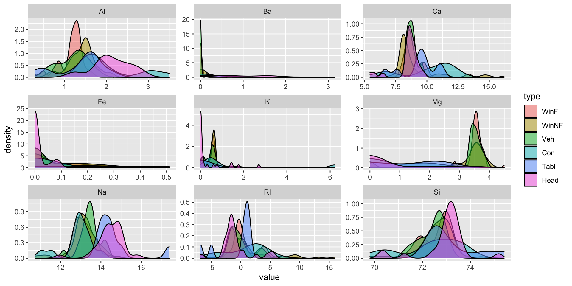
In this dataset, it is difficult to see distinctions between the six different types of glass. The distributions of measurements for each type of glass and each element measurement overlap significantly. In the Mg measurements, there appear to be two distinct groups: WinF, WinNF, and Veh in one group, and Con, Tabl, and Head glass in another group. The first group has higher values of Mg and has less variability in Mg values than the second group.
We can also look at numerical summaries of the data. Below, each entry is (mean, sd) of the measurements on the variable.
| type | Al | Ba | Ca | Fe | K | Mg | Na | RI | Si |
|---|---|---|---|---|---|---|---|---|---|
| WinF | (1.16,0.27) | (0.01,0.08) | (8.8,0.57) | (0.06,0.09) | (0.45,0.21) | (3.55,0.25) | (13.24,0.5) | (0.72,2.27) | (72.62,0.57) |
| WinNF | (1.41,0.32) | (0.05,0.36) | (9.07,1.92) | (0.08,0.11) | (0.52,0.21) | (3,1.22) | (13.11,0.66) | (0.62,3.8) | (72.6,0.72) |
| Veh | (1.2,0.35) | (0.01,0.04) | (8.78,0.38) | (0.06,0.11) | (0.41,0.23) | (3.54,0.16) | (13.44,0.51) | (-0.04,1.92) | (72.4,0.51) |
| Con | (2.03,0.69) | (0.19,0.61) | (10.12,2.18) | (0.06,0.16) | (1.47,2.14) | (0.77,1) | (12.83,0.78) | (0.93,3.35) | (72.37,1.28) |
| Tabl | (1.37,0.57) | (0,0) | (9.36,1.45) | (0,0) | (0,0) | (1.31,1.1) | (14.65,1.08) | (-0.54,3.12) | (73.21,1.08) |
| Head | (2.12,0.44) | (1.04,0.67) | (8.49,0.97) | (0.01,0.03) | (0.33,0.67) | (0.54,1.12) | (14.44,0.69) | (-0.88,2.55) | (72.97,0.94) |
It’s clear from this table that only tableware glass lacks Ba, Fe, and K. Furthermore, we may be able distinguish between container glass and headlamp glass because container tends to have higher levels of K and lower levels of Ba than headlamp glass. It still looks like WinF, WinNF and Veh glass are not easily distinguishable based on the data in this table.
CSAFE data: Next, we look at the data collected for CSAFE. I take a look and 4 panes, 2 from Manufacturer A, and 2 from Manufacturer B. There are more elements available on this data than on the previous data, and they are measured on a different scale (ppm). In the figure below, can you determine which 2 panes came from A and which 2 came from B?
glass <- read_csv("dat/glass_sample.csv")
glass2 <- glass %>% gather(variable, value, Li7:Pb208)

ggplot(data = glass2) +
  geom_density(aes(x = value,fill = pane), alpha = .5) +
  facet_wrap(~variable, scales="free") +
  scale_fill_brewer(palette = "Set2") +
  labs(x = "concentration in ppm")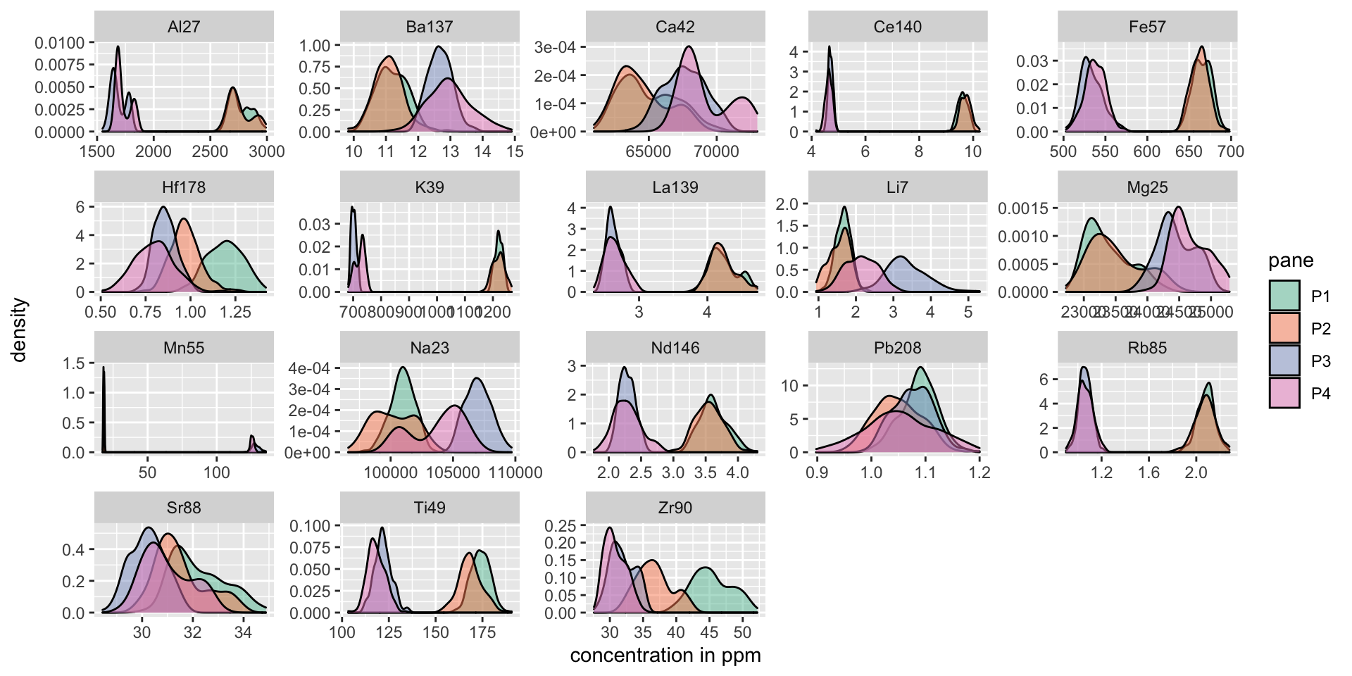
Pane1 and Pane2 are from Manufacturer A and Pane3 and Pane4 are from Manufacturer B. These two manufacturers, in the complete dataset, can be perfectly distinguished by only one measurement: that of K39, the ppm measurement of potassium in the glass. To distinquish between the panes, we can fit a random forest using the R package randomForest.
glass2.1 <- glass2 %>% spread(variable, value) %>% dplyr::select(-Piece, -Rep, -mfr) %>% mutate(row = row_number()) %>% mutate_if(is.numeric, log)
set.seed(345892)
glass2.1test <- glass2.1 %>% sample_n(100)
glass2.1train <- glass2.1 %>% filter(!(row %in% glass2.1test$row))
rf1 <- randomForest(as.factor(pane)~., data=glass2.1train[,-20], xtest = glass2.1test[,-c(1,20)], ytest = as.factor(glass2.1test$pane), importance=T, ntree=1000, keep.forest = T)
rf1
##
## Call:
## randomForest(formula = as.factor(pane) ~ ., data = glass2.1train[, -20], xtest = glass2.1test[, -c(1, 20)], ytest = as.factor(glass2.1test$pane), importance = T, ntree = 1000, keep.forest = T)
## Type of random forest: classification
## Number of trees: 1000
## No. of variables tried at each split: 4
##
## OOB estimate of error rate: 0.18%
## Confusion matrix:
## P1 P2 P3 P4 class.error
## P1 137 0 0 0 0.000000000
## P2 0 136 0 0 0.000000000
## P3 0 0 137 1 0.007246377
## P4 0 0 0 149 0.000000000
## Test set error rate: 0%
## Confusion matrix:
## P1 P2 P3 P4 class.error
## P1 28 0 0 0 0
## P2 0 29 0 0 0
## P3 0 0 27 0 0
## P4 0 0 0 16 0glass2.1$pred1 <- predict(rf1, glass2.1[,-c(1,20)])
table(glass2.1$pred1, glass2.1$pane)##
## P1 P2 P3 P4
## P1 165 0 0 0
## P2 0 165 0 0
## P3 0 0 165 0
## P4 0 0 0 165varImpPlot(rf1)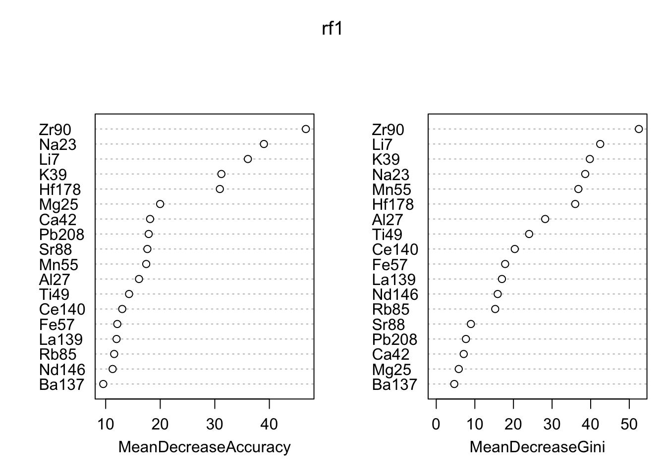
Using a random forest, we are able to discriminate almost perfectly between the four panes. The function randomForest::varImpPlot shows the importance of each of the 18 elements in the data set. The two “most important” variables according to both metrics are Zr90 and Li7. The plot below shows the relationship between those two. We can see the groups are pretty well separated.
ggplot(data = glass2.1, aes(x=Zr90, y=Li7)) +
  geom_point(aes(color = pane)) +
  scale_color_brewer(palette = "Set2") +
  labs(x = "log(Zr90) (ppm)", y = "log(Li7) (ppm)")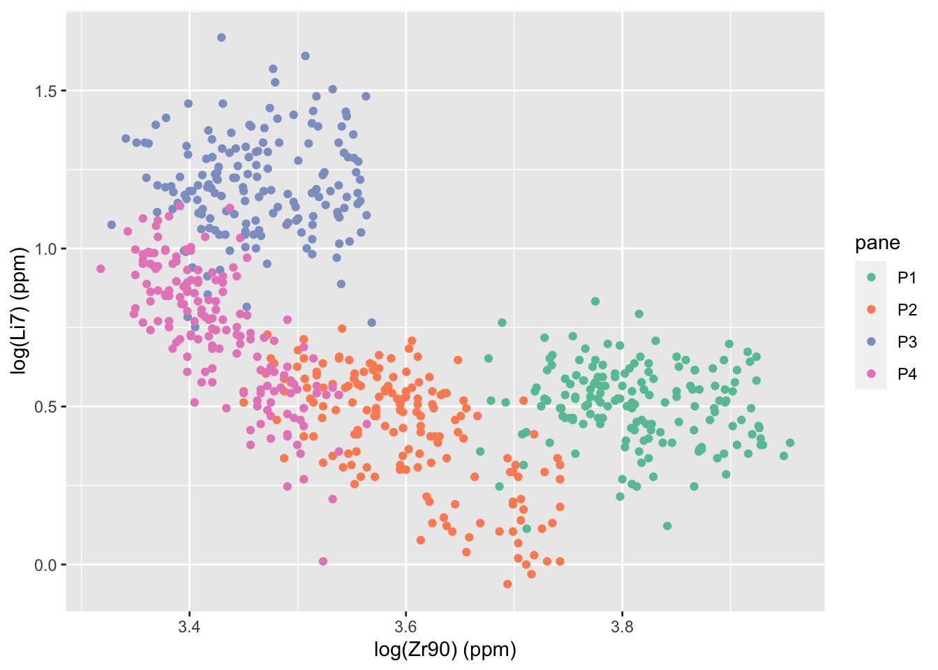
Next, we can build a random forest on only the two most important variables, to see where the regions of classification are and to see where the random forest fails. We only allow each tree in the forest to have 4 nodes to avoid overfitting.
glasstrain2 <- glass2.1train[,c("pane","Zr90", "Li7")]
glasstest2 <- glass2.1test[,c("pane","Zr90", "Li7")]
rf2 <- randomForest(as.factor(pane) ~ ., data = glasstrain2, xtest = glasstest2[,-1], ytest = as.factor(glasstest2$pane), ntree=500, keep.forest = T, mtry = 2, maxnodes=4)
rf2
##
## Call:
## randomForest(formula = as.factor(pane) ~ ., data = glasstrain2, xtest = glasstest2[, -1], ytest = as.factor(glasstest2$pane), ntree = 500, keep.forest = T, mtry = 2, maxnodes = 4)
## Type of random forest: classification
## Number of trees: 500
## No. of variables tried at each split: 2
##
## OOB estimate of error rate: 25.89%
## Confusion matrix:
## P1 P2 P3 P4 class.error
## P1 124 13 0 0 0.09489051
## P2 6 27 0 103 0.80147059
## P3 0 0 125 13 0.09420290
## P4 0 0 10 139 0.06711409
## Test set error rate: 28%
## Confusion matrix:
## P1 P2 P3 P4 class.error
## P1 28 0 0 0 0.00000000
## P2 0 4 0 25 0.86206897
## P3 0 0 25 2 0.07407407
## P4 0 0 1 15 0.06250000zr90r <- range(glass2.1$Zr90)
Li7r <- range(glass2.1$Li7)
newdata <- expand.grid(Zr90 = seq(zr90r[1],zr90r[2],length.out = 500),
Li7 = seq(Li7r[1],Li7r[2],length.out = 500))
newdata$pred2 <- predict(rf2, newdata)
ggplot() +
geom_tile(data = newdata, aes(x = Zr90, y = Li7, fill = pred2), alpha = .4) +
geom_point(data = glass2.1, aes(x = Zr90, y = Li7, color = pane)) +
scale_color_brewer(palette = "Set2") +
scale_fill_brewer(palette = "Set2") +
labs(x = "log(Zr90) (ppm)", y = "log(Li7) (ppm)")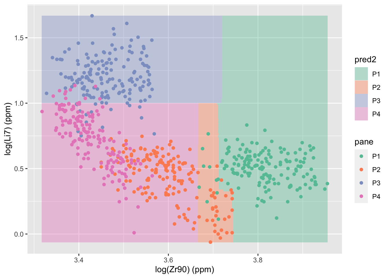
These analyses are informative about glass generally, for instance if we want to determine manufacturer of a window, but are less helpful when making forensic comparisons. In the practical forensic application, there is only one known pane and some fragments from an unknown source. The goal is to determine if the fragments come from the known pane, so a more generic “matching” approach is necessary. This approach will be covered in a future post.
References
Curran, James Michael, Tacha Natalie Hicks, and John S. Buckleton. 2000. Forensic Interpretation of Glass Evidence. CRC Press.
R. Cook, Evett, I.W., Jackson, G., Jones, P.J., and Lambert, J.A. (1998) “A hierarchy of propositions: deciding which level to address in casework.” Science and Justice. 38:4 pp 231-239.
ASTM International, ASTM E2330-12 Standard Test Method for Determination of Concentrations of Elements in Glass Samples Using Inductively Coupled Plasma Mass Spectrometry (Icp-Ms) for Forensic Comparisons. 2012. West Conshohocken, PA, ASTM International. doi: https://doi.org/10.1520/E2330-12.
Weis, Peter, Marc Ducking, Peter Watzke, Sonja Menges, and Stefan Becker. 2011. “Establishing a Match Criterion in Forensic Comparison Analysis of Float Glass Using Laser Ablation Inductively Coupled Plasma Mass Spectrometry.” Journal of Analytical Atomic Spectrometry. 26 (6). The Royal Society of Chemistry: 1273–84. doi:10.1039/C0JA00168F.
Venables, W. N. and Ripley, B. D. (2002) Modern Applied Statistics with S. Fourth edition. Springer.
Newman, D.J. & Hettich, S. & Blake, C.L. & Merz, C.J. (1998). UCI Repository of machine learning databases [http://www.ics.uci.edu/~mlearn/MLRepository.html]. Irvine, CA: University of California, Department of Information and Computer Science.
Friedrich Leisch & Evgenia Dimitriadou (2010). mlbench: Machine Learning Benchmark Problems. R package version 2.1-1.
Hadley Wickham (2017). tidyverse: Easily Install and Load the ‘Tidyverse’. R package version 1.2.1. https://CRAN.R-project.org/package=tidyverse
A. Liaw and M. Wiener (2002). Classification and Regression by randomForest. R News 2(3), 18–22.
Sam Tyner-Monroe, Ph.D.
Managing Director, Responsible AI
I am an applied statistician and data scientist, with a wide range of skills and experiences. I’m passionate about using data to make a difference.