Forensic Glass Analysis - Part II

Aug 24, 2018 blog, rstats, forensics, glass

This post is the second of two on the forensic analysis of glass evidence. The first post discusses the background problem, the manufacture of glass, and the format of the data for statistical analyses. Start there!

Source conclusions: previous work

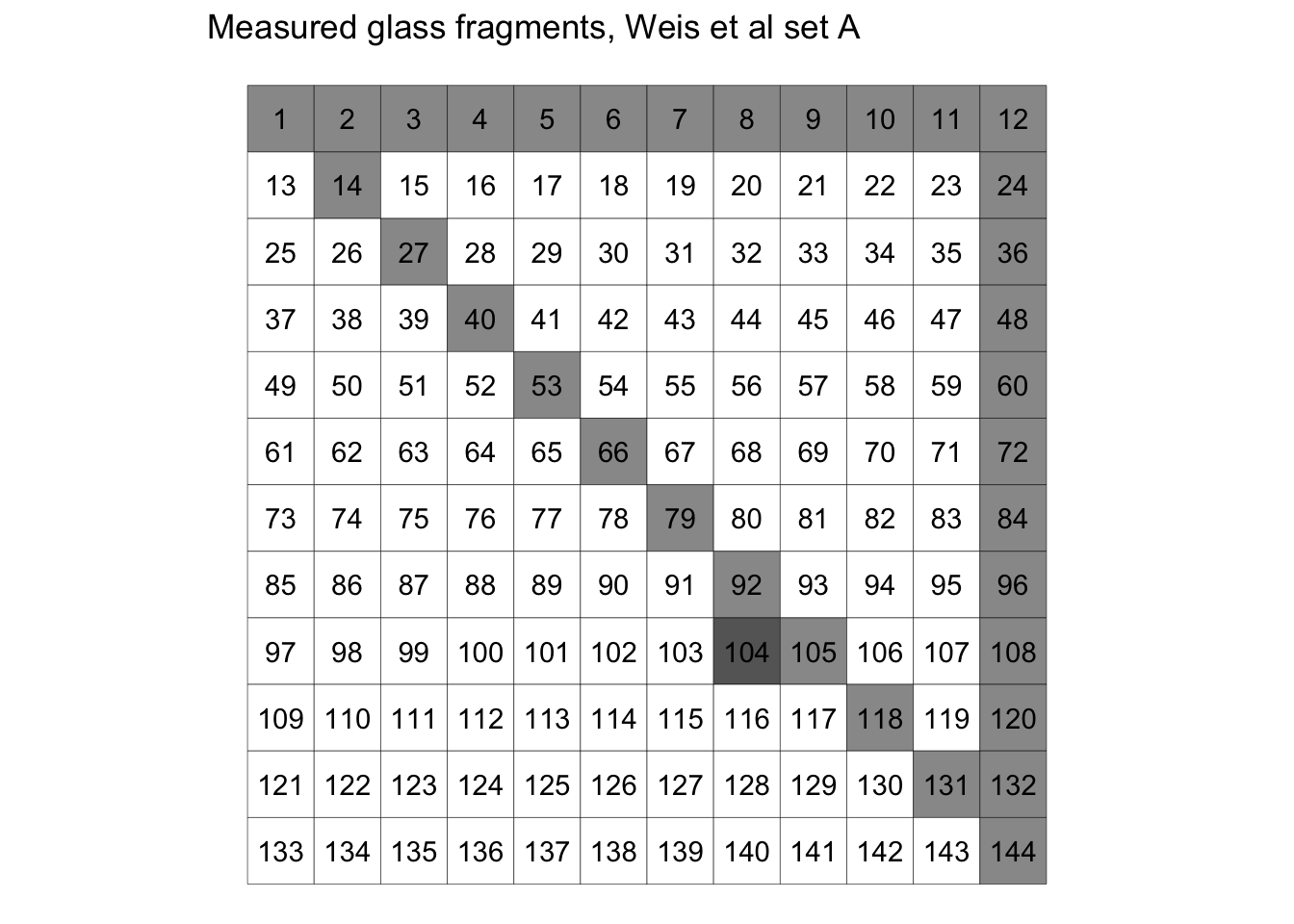
Weis et al (2011) introduced several criteria for determining whether two glass fragments came from the same source [1]. They had 2 sets of glass data. The first set, set A, consited of 33 fragments of glass from the same pane measured 6 times each, plus one additional fragment measured 11 different times, for a total of 44 measurements. These fragments are shown in the figure below, where the whole grid represents a pane of glass, and the fragments are the numbered tiles within the pane. The 44 measurements were collected over 11 days. Three of the 33 fragments were sampled on each day and measured 6 times. On every day, the 34th fragment was measured 6 times on all 11 days. So, there are 6 measurements from all gray tiles in the figure below except for tile 104. From tile 104 there are 66 total measurements from 11 different days. Each replicate is a vector of 18 element concentrations: Li, Na, Mg, Al, K, Ca, Ti, Mn, Fe, Rb, Sr, Zr, Ba, La, Ce, Nd, Hf, Pb.

The second set of measurements, Dataset B, are measurements on 62 panes of float glass from 18 different companies, of three different colors. The 62 panes were measured 6 times each, for a total of 372 measurements. The companies were in 8 different countries: Brazil, Finland, Germany, Italy, Japan, Spain, Sweden, and the United States.

The 6 repetitions from each are averaged, and pairwise comparison of the average measurements of each element are done for all possible pairs in each data set. There are $44 * 43 = 1892 $ comparisons for dataset A and $62*61 = 3782 $ comparisons for dataset B. According to the criteria defined, a source conclusion is made based on the pairwise comparisons of each element measurement in glass. The conclusion is “different source” if any one or more of the 18 elements fails the match criteria.

Errors

There are two types of error to be made in Weis et al., Type I and Type II. A type I error, also called a “false negative” in Weis et al., is when the conclusion “different source” is made when the truth is “same source”. Think of a type I error here as “failing to convict a guilty person”. A type II error, also called a “false positive” in Weis et al., is when the conclusion “same source” is made when the truth is “different source”. Think of the Type II error here as “convicting an innocent person”.

	Conclusion
Truth	Same Source	Different Source
Same Source	✓	Type I error (false negative)
Different Source	Type II error (false positive)	✓

All of the Type I errors are computed with respect to dataset A, which all come from the same pane of glass, while all of the Type II errors are computed with respect to dataset B, where all measurements are from different different panes of glass. Since it is generally considered worse to convict an innocent person than to fail to convict a guilty person, the Type II error here has lower tolerance than Type I error.

What is a “match”? (Previous work)

Weis et al define five distinct criteria for determining a match between two glass samples.

The first is the “$n$-Sigma criterion I”. Here a “match” is declared between fragment A and fragment B if the means of all 18 element measurements in fragment B fall within the interval $\mu_{Ai} \pm n\times \sigma_A$ where $\mu_{Ai}$ is the observed mean measurement of element $i$ in fragment A, and $\sigma_A$ or “sigma” is the standard deviation of the 6 measurements of fragment A. The value $n$ is an integer, $n = 1, 2, 3, \dots$, and Weis et all determined the best $n$, in terms of balancing the Type I and Type II error rates is $n = 10$. So, a “match” is delcared if the mean of measurements from fragment B fall within $10 \times \sigma_A$ of the mean values from fragment A. (Type I & Type II errors occur 15.17% and 0.13% of the time, respectively, for $n=10$ and the data collected by Weis et al.)
The second criterion is the “$n$-Sigma criterion II”. Here, a “match” is declared if the $n$-sigma intervals around the means of both fragment A and fragment B overlap. In other words, if the intervals $\mu_{Ai} \pm n\times \sigma_A$ and $\mu_{Bi} \pm n\times \sigma_B$ intersect at all for all 18 elements, a “match” is declared. A “non-match” is declared if any one of the 18 pairs of intervals do not overlap. (Type I & Type II errors occur 0% and 0.58% of the time, respectively, for $n=10$ and the data collected by Weis et al.)
The third criterion is called the “Modified $n$ sigma criterion with fixed relative standard deviations”. The difference between this method and the other two methods is that the “sigma” that is used is derived from 90 values computed from 90 observations of 3 replicates each from the German glass standard DGG1. The standard deviation of elementh measurements from the 90 values is called the “fixed relative standard deviations” (FRSD). If the value of the FRSD for an element is less than 3%, it is set to 3%. The interval computed is $(\frac{\mu_{Ai}}{1+ n \times FRSD} , \mu_{Ai}\times (1+ n\times FRSD))$. The interval is used as in 1., where if at least one mean value from fragment B does not fall in the interval from fragment A, a “non-match” is declared. (Type I & Type II errors occur 1.04% and 0.11% of the time, respectively, for $n=4$ and the data collected by Weis et al.)
The fourth criterion is the Student’s $t$-test for equal means for each of the 18 elements with a Bonferroni correction. Thus, the crierion is based on the chosen type I error rate, $\alpha$, and the Bonferroni correction means that the hypothesis of identical means of one element is rejected if the test statistic is larger than $t_{1-1/2 \cdot \alpha/18}$ for 10 degrees of freedom. The test statistic uses the means and standard deviations for each element within a fragment. (For $\alpha = 0.05$, the Type I & Type II error rates were 91.12% and 0%, respectively.)
The fifth and final criterion is also a $t$-test with Bonferroni correction, but the FRSD is used in place of the standard deviations of each of the 6 repeated measures. (For $\alpha = 0.05$, the Type I & Type II error rates were 36.36% and 0%, respectively.)

Ultimately, Weis et al conclude that the modified 4 sigma criterion (#3) is the best one, and they say is has been applied in casework and used in over 70 court cases. (Though they don’t explicity say where the cases were, it is safe to assume that the method has only been applied in Germany, as Weis’ affiliation is the Forensic Science Institute in Wiesbaden, Germany.)

Source Conclusions: Current CSAFE work

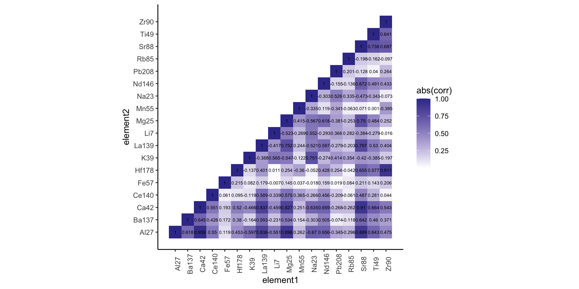
The previous methods described do not take into account the correlations between element measurements. In addition, as the variablility of measurements of one or more elements increase within a pane, it is increasingly harder to reject the null hypothesis (that two fragments have the same source). This has implications in the courtroom: higher variability would tend to incriminate the defendant because the intervals of Weis et al would tend to be wider, and the null hypothesis not disproven. CSAFE researchers have developed a new method using scores derived from supervised machine learning methods such as random forest (RF) and Bayesian additive regression trees (BART). The scores take into account all 18 elemental measurements of the glass together and can account for the known relationships (linear and non-linear) between elemental concentrations. Consider, for example, the absolute correlation matrix shown below for the elements from Manufacturer 1. Correlations with absolute value near 1 are colored dark blue, while correlations near 0 colored white. As you can see, there are several off-diagonal pairs above 0.9, indicating strong relationships between those elements.

The previous methods do not incorporate this correlation information into their decision making process. In addition, the algorithms used by CSAFE researchers provide a ranking of the variables that are most discriminating when determining whether the glass fragments have the same or different sources. Finally, the algorithms compute the probability (the score) that the pair of fragments have the same source or a different source. The application of machine learning techniques to glass element analysis outperforms the traditional interval methods by keeping both the Type I and Type II error rates low, whereas the interval methods tend to have one very low and the other unacceptably high.

The results discussed above are submitted to the Annals of Applied Statistics by Park and Carriquiry.

References

Weis, Peter, Marc Ducking, Peter Watzke, Sonja Menges, and Stefan Becker. 2011. “Establishing a Match Criterion in Forensic Comparison Analysis of Float Glass Using Laser Ablation Inductively Coupled Plasma Mass Spectrometry.” Journal of Analytical Atomic Spectrometry. 26 (6). The Royal Society of Chemistry: 1273–84. doi:10.1039/C0JA00168F.
Hadley Wickham (2017). tidyverse: Easily Install and Load the ‘Tidyverse’. R package version 1.2.1. https://CRAN.R-project.org/package=tidyverse

Sam Tyner-Monroe, Ph.D.

Managing Director, Responsible AI

I am an applied statistician and data scientist, with a wide range of skills and experiences. I’m passionate about using data to make a difference.